In Appendixes some particular hypotheses will be considered. Practically, they do not connected with the criticism of relativity theory from the main part of this book; they only demonstrate nonuniqueness of the SRT approach and a possibility of the frequency parametrization of all formulas. This is the only claim of these appendixes in the book, since we will use incorrect SRT methods (their error was proved in the main part of the book). The author attempted to discuss ideas from Appendixes A and B (plus a part of analysis of the Michelson experiment from Chapter 3) in several well-known journals in 1993-1999. The result was the same: either the work did diplomatically not be considered right away or the approximate answer was "nobody discovered these things in relativity theory and quantum electrodynamics, but the exactness of predictions of these theories was huge". How can theorist discover anything new (instead of explanation its "by late mind")? He must assume some fact and test corollaries from his assumption. But nobody attempts to assume the possibility of frequency dependence of light speed. Besides, the case in point was the precision on one-two orders large than the existing modern precision of experiments. Such a precision can be reached in the immediate future; though there exist experiments, which need in precision on some dozens of orders large than existing one, but they have been seriously discussing in physics. The author was tired to waste the time at last, and a decision was taken to test the "huge precision of relativity theory" (at the same time remembering a student dissatisfaction by this theory). As a result, my first critical article appeared (and now this book too). So, plus and minus together are presented everywhere.
Now we proceed to discussion of a possible frequency dependence of light speed.
It is well known that when particles are in vacuum, there occur
various processes, such as the appearance of
virtual pairs (a particle and
its antiparticle); many interaction processes are
described in terms of such virtual pairs. Also, light influences
vacuum properties during its propagation (in particular,
vacuum polarization takes place). Therefore, by the reciprocity principle
there must
be a reverse action of vacuum polarization on the light propagation.
As a consequence, the light (at a certain frequency) is bound to
travel through the vacuum as "the medium" with some certain permittivity
![]() , which is determined by this light itself;
that is,
, which is determined by this light itself;
that is, ![]() .
.
The generalization of the Maxwell equations by adding the mass term explicitly
to the Maxwell Lagrangian is known to lead to the Proca equations in the
Minkowski space (in the modern view). An electromagnetic wave propagating
through the medium is influenced by the latter and this effect is manifested via
the generation of massive photons [100]. Even with constant phase speed assumed,
an ![]() -dependence of the
group speed (dispersion in vacuum) is known to
arise:
-dependence of the
group speed (dispersion in vacuum) is known to
arise: ![]() , where
, where ![]() is the
rest mass of the photon. However, the
question of mass generation and the
gauge theories will not be discussed in
these Appendixes. Our aim is just to
represent some physical reflections about light velocity and attendant questions.
is the
rest mass of the photon. However, the
question of mass generation and the
gauge theories will not be discussed in
these Appendixes. Our aim is just to
represent some physical reflections about light velocity and attendant questions.
The questions arise here: 1) How can the ![]() -dependence be evaluated or
measured? 2) Why has it not yet been found, and 3) What corollaries follow?
-dependence be evaluated or
measured? 2) Why has it not yet been found, and 3) What corollaries follow?
There exist various methods for measuring light speed:
astronomical methods,
the method of interruptions, the rotating
mirror method, the radio geodetic
method, the method of standing waves (the resonator),
the independent
measurements of ![]() and
and ![]() , and so on. At the present time, the last
method [59,67] is the most precise; it is used by the Bureau of Standards for
measuring light speed to eight significant digits. However, an important problem
arises in this approach [7]. Besides, it must be emphasized that this method is
principally limited: either it can be connected with local (inside a device)
speed of light only, or it can bear no relationship to light speed at all in the
case if light by itself does not represent a pure wave.
Why other methods are inadequate (fail to detect
, and so on. At the present time, the last
method [59,67] is the most precise; it is used by the Bureau of Standards for
measuring light speed to eight significant digits. However, an important problem
arises in this approach [7]. Besides, it must be emphasized that this method is
principally limited: either it can be connected with local (inside a device)
speed of light only, or it can bear no relationship to light speed at all in the
case if light by itself does not represent a pure wave.
Why other methods are inadequate (fail to detect ![]() dependence) is
clear from the previous Chapters and will be clear from given Appendixes for
one particular hypothesis.
dependence) is
clear from the previous Chapters and will be clear from given Appendixes for
one particular hypothesis.
In further consideration we will follow SRT methods (we will forget their error
for the time being, but present an "apparent effect" for two systems under an
additional condition only - under the condition of the choice of the Einstein
synchronization method).
Recall that in deriving the corollaries of SRT (transformation laws, for
example) the notion of the interval ![]() is used.
Here it is necessary to make two methodological remarks. First, even the
equality of intervals
is used.
Here it is necessary to make two methodological remarks. First, even the
equality of intervals ![]() is nothing more than one possible
hypotheses, since only a single point
is nothing more than one possible
hypotheses, since only a single point ![]() remains
trustworthy (if we suppose
remains
trustworthy (if we suppose ![]() ). For example, we could pick any
natural number
). For example, we could pick any
natural number ![]() and equate the
and equate the ![]() degrees,
degrees,
![]() , and obtain different "physical laws". Or,
we could consider
, and obtain different "physical laws". Or,
we could consider ![]() , but
, but ![]() , i.e.
, i.e.
![]() (the apparent velocity of mutual motion is different
for different observers). Such a choice results in coinciding of the
relativistic longitudinal Doppler effect with the classical expression. Similar
exotic systems could be as much intrinsically self-consistent as the SRT (i.e.
for two marked objects only!), and only the experiments
could demonstrate which choices are nothing more than theoretical
fabrications. We shall not discuss all such exotic hypotheses here.
(the apparent velocity of mutual motion is different
for different observers). Such a choice results in coinciding of the
relativistic longitudinal Doppler effect with the classical expression. Similar
exotic systems could be as much intrinsically self-consistent as the SRT (i.e.
for two marked objects only!), and only the experiments
could demonstrate which choices are nothing more than theoretical
fabrications. We shall not discuss all such exotic hypotheses here.
Second, in the usage of interval, the following point is not emphasized: the specific
light, propagating from one point to another, is used in this case,
i.e. the value ![]() should be substituted in the
expression for the interval. But in such a case, assuming proportionality
of intervals from textbooks, an indeterminate relation is obtained:
should be substituted in the
expression for the interval. But in such a case, assuming proportionality
of intervals from textbooks, an indeterminate relation is obtained:
and even the equality of intervals cannot be proved.
This indeterminate relation is associated with the still "unknown" Doppler law,
so there is again need for reference to experiments. Thus,
theoretical constructions proceeding from intrinsic individual principles
are not unique. Since generally accepted derivations results in some
corollaries that are confirmed experimentally (for particle dynamics
within some precision, for example), we shall rely upon this method, but
modify it with regard to the possible ![]() dependence.
dependence.
Physically, this approach implies the following: The apparent result of some
measurement depends on the measurement technique; and the calculated result
depends,in particular, on the synchronization procedure
for timepieces in
different frames. According to an idea from this Appendix, no "unique
interaction propagation speed" exists (but ![]() ). If
light of some
definite frequency
). If
light of some
definite frequency ![]() is used for Einstein synchronization of timepieces
in the different
frames, the result of any
experiment depends on
is used for Einstein synchronization of timepieces
in the different
frames, the result of any
experiment depends on ![]() . For
example, if some process with characteristic
. For
example, if some process with characteristic ![]() takes place
in a system,
then it is natural to watch the system by using
takes place
in a system,
then it is natural to watch the system by using
![]() (just as the
signal propagates).
If two systems moving
relative to each other are studied in the experiment,
then two quantities
(just as the
signal propagates).
If two systems moving
relative to each other are studied in the experiment,
then two quantities
![]() and
and ![]() (for each frame) appear
in formulae. This is due to
the fact, that the same light possesses
different frequencies in systems
moving relative to each other.
As this takes place, the quantities
(for each frame) appear
in formulae. This is due to
the fact, that the same light possesses
different frequencies in systems
moving relative to each other.
As this takes place, the quantities ![]() and
and ![]() are related
to each other by the Doppler effect (see below). It
is interesting to note
the following circumstance. If several various
processes with characteristic
frequencies
are related
to each other by the Doppler effect (see below). It
is interesting to note
the following circumstance. If several various
processes with characteristic
frequencies ![]() take place in the system,
then the observers moving
with respect to each other will see (at the
same point) various pictures of events (the apparent effect). In the subsequent
theoretical description we shall follow [4,17].
take place in the system,
then the observers moving
with respect to each other will see (at the
same point) various pictures of events (the apparent effect). In the subsequent
theoretical description we shall follow [4,17].
Let ![]() be the frequency of signal
propagation in some system. Substituting
be the frequency of signal
propagation in some system. Substituting ![]() (instead of
(instead of ![]() ) into the
four-dimensional interval
) into the
four-dimensional interval ![]() for the intrinsic system and
for the intrinsic system and ![]() into
into ![]() for the system of observation, it
follows from
for the system of observation, it
follows from ![]() that the intrinsic time (
that the intrinsic time (![]() ) can be found from
) can be found from
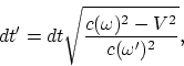 |
(A.1) |
but the formula for the intrinsic length retains its validity. We note again, that it is "a visible effect" only. In an arbitrary mathematical expression coefficients can be transfered (according to some rules) from the left-hand side in the right-hand side of the expression and vice versa (all these expressions are equivalent). Then, how can it be determined: accelerats time at one observer or, contrary, decelerats at other one (and increased or decreased lengths)? Simply, if somebody were said to you that just yours time is decelerated by different manner relative several objects, you would right away understand senselessness of the infinite number of such "informations". However relativists say that yours time is OK, but simply "somebody has something somewhere far off", and many people calm right away and continue to listen "the fairy-tales".
To derive the Lorentz transformations, one can use rotation in the ![]() plane:
plane:
Using ![]() , it follows that the Lorentz
transformation reduces to
, it follows that the Lorentz
transformation reduces to
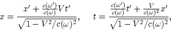 |
(A.2) |
where ![]() is the system velocity.
Writing
is the system velocity.
Writing ![]() and
and ![]() in the expression (A.2) and finding
in the expression (A.2) and finding ![]() ,
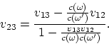
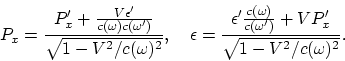
one obtains, that the transformations for velocity change into
,
one obtains, that the transformations for velocity change into
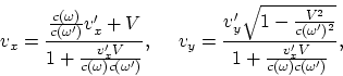
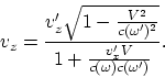 |
(A.3) |
It follows that for the motion along the ![]() axis
axis
 |
(A.4) |
We see that the maximum of velocity is ![]() ,
where
,
where ![]() is the light frequency in the intrinsic system. Note that all
formulae lead to the correct composition law for motion along the same straight
line (the transformation from frame
is the light frequency in the intrinsic system. Note that all
formulae lead to the correct composition law for motion along the same straight
line (the transformation from frame ![]() to
to ![]() and from
and from ![]() to
to ![]() yields the
same result as the transformation
from
yields the
same result as the transformation
from ![]() to
to ![]() ). Recall that, in accord with
considerations given in the main part of the book, quantities
). Recall that, in accord with
considerations given in the main part of the book, quantities ![]() and
and ![]() in
formulas (A.1), (A.2) have no intrinsic physical meaning (they are fictitious
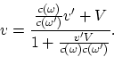
auxiliary quantities). Formula (A.4),
by analogy with formula (1.5), can be re-written as
in
formulas (A.1), (A.2) have no intrinsic physical meaning (they are fictitious
auxiliary quantities). Formula (A.4),
by analogy with formula (1.5), can be re-written as
 |
(A.5) |
This form most clearly reveals the essence of this expression (the apparent
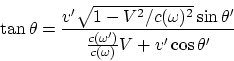
effect). The formula
 |
(A.6) |
describes the change of the velocity direction. The relativistic expression
for the light aberration holds (the substitution ![]() ). To be on the safe side, we are reminded that the
relativistic expression for the stellar aberration is approximate. The
transformations of 4-vectors are also valid. From here follow the
transformations of the wave four-vector
). To be on the safe side, we are reminded that the
relativistic expression for the stellar aberration is approximate. The
transformations of 4-vectors are also valid. From here follow the
transformations of the wave four-vector ![]() :
:
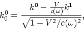
As a result, the Doppler effect can be obtained from
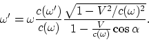 |
(A.7) |
Note, that from here follows the dependence of light speed on the system
motion (different frequencies ![]() correspond to different systems).
However, as we shall see in the next Appendix, this effect is negligible for the
visible region. Relativists declare that the expression of the Doppler effect contains the relative
velocity. It is false. Let an explosion occur at some point on the Earth, and let some
line of emission be radiated in short time. Let a receiver at the Pluton catch the signal. At
which a moment must we determine this mythical relative velocity? The receiver can not see
in the direction to the Earth at the moment of explosion, and the source not exists at the
moment of the signal receiving, and the Earth will be turned to the back side. Even in the
absence of medium, we obtain, instead of the relative velocity, the difference of absolute
velocities at the moment of emission and at the moment of signal receiving (and it is not
the same!). But the real result can be obtained in the real experiment only.
correspond to different systems).
However, as we shall see in the next Appendix, this effect is negligible for the
visible region. Relativists declare that the expression of the Doppler effect contains the relative
velocity. It is false. Let an explosion occur at some point on the Earth, and let some
line of emission be radiated in short time. Let a receiver at the Pluton catch the signal. At
which a moment must we determine this mythical relative velocity? The receiver can not see
in the direction to the Earth at the moment of explosion, and the source not exists at the
moment of the signal receiving, and the Earth will be turned to the back side. Even in the
absence of medium, we obtain, instead of the relative velocity, the difference of absolute
velocities at the moment of emission and at the moment of signal receiving (and it is not
the same!). But the real result can be obtained in the real experiment only.
The energy-momentum vector transforms as
 |
(A.8) |
There should be a closer analogy between light propagation through vacuum and through a medium.
1) Various packets of waves diffuse in vacuum variously.
2) Light dispersion in vacuum imposes a fundamental limitation on the degree of ray parallelism.
3) There is light dissipation in vacuum; that is, the intensity of light decreases as it propagates in vacuum.
4) Light "ages"; that is, the frequency of light decreases as it propagates in vacuum. This phenomenon bears on the paradox (Olbers) "why does the sky not flame?" and contributes to the red shift; that is, a correction of the world evolution concept is in order. Since we are factually dealing with an alternative explanation of the red shift, this effect appears to be very small, and, at present, it cannot be confirmed in laboratoty experiments: the red shift of lines for cosmic objects is already detected by the most precise optical methods and it becomes to be noticeable for very distant objects only, such the ones that distances to theirs cannot be found even on the Earth's orbit base (on the triangle). Recall in this connection that even an order of the value of Habble constant had already been corrected.
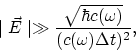
Passing to quantum electrodynamics, the substitution ![]() needs to be done in all derivations. For example, this dependence appears in
the uncertainty relation
needs to be done in all derivations. For example, this dependence appears in
the uncertainty relation
in the condition for classical description
and in numerous formulae.
If some formula describes the ![]() -dependence, then
it can substantially change. As an example, we consider the emission and
absorption of photons. The new coefficient
-dependence, then
it can substantially change. As an example, we consider the emission and
absorption of photons. The new coefficient
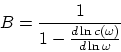
appears in the expression for the number ![]() of photons
with a given polarization:
of photons
with a given polarization:
and in the relation for probabilities (of absorption, induced and spontaneous
emission) ![]() .
Quantity
.
Quantity ![]() appears in Einstein's coefficients.
appears in Einstein's coefficients.
Using the substitution ![]() for natural field
oscillations, one obtains the expression for the Fourier component of the
photon propagator:
for natural field
oscillations, one obtains the expression for the Fourier component of the
photon propagator:
We cannot find ![]() without knowledge of the explicit
dependence
without knowledge of the explicit
dependence ![]() . The explicit form of the
. The explicit form of the ![]() -dependence is
necessary to find a net result for various cross-sections (for scattering,
for the origin of a pair, for disintegration, etc.).
As a first approximation, the substitution
-dependence is
necessary to find a net result for various cross-sections (for scattering,
for the origin of a pair, for disintegration, etc.).
As a first approximation, the substitution ![]() can be made
in the well-known formulae.
can be made
in the well-known formulae.
There we shall discuss the possible ![]() -dependence.
-dependence.